Data Definition
Data Definition defines a particular data with the following characteristics.
Atomic − Definition should define a single concept.
Traceable − Definition should be able to be mapped to some data element.
Accurate − Definition should be unambiguous.
Clear and Concise − Definition should be understandable.
Data Object
Data Object represents an object having a data.
Data Type
Data type is a way to classify various types of data such as integer, string, etc. which determines the values that can be used with the corresponding type of data, the type of operations that can be performed on the corresponding type of data. There are two data types −
- Built-in Data Type
- Derived Data Type
Built-in Data Type
Those data types for which a language has built-in support are known as Built-in Data types. For example, most of the languages provide the following built-in data types.
- Integers
- Boolean (true, false)
- Floating (Decimal numbers)
- Character and Strings
Derived Data Type
Those data types which are implementation independent as they can be implemented in one or the other way are known as derived data types. These data types are normally built by the combination of primary or built-in data types and associated operations on them. For example −
- List
- Array
- Stack
- Queue
Basic Operations
The data in the data structures are processed by certain operations. The particular data structure chosen largely depends on the frequency of the operation that needs to be performed on the data structure.
- Traversing
- Searching
- Insertion
- Deletion
- Sorting
- Merging
Array is a container which can hold a fix number of items and these items should be of the same type. Most of the data structures make use of arrays to implement their algorithms. Following are the important terms to understand the concept of Array.
Element − Each item stored in an array is called an element.
Index − Each location of an element in an array has a numerical index, which is used to identify the element.
Array Representation
Arrays can be declared in various ways in different languages. For illustration, let's take C array declaration.

Arrays can be declared in various ways in different languages. For illustration, let's take C array declaration.
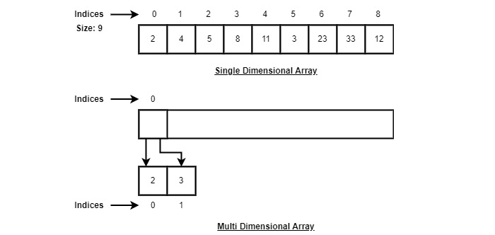
As per the above illustration, following are the important points to be considered.
Index starts with 0.
Array length is 10 which means it can store 10 elements.
Each element can be accessed via its index. For example, we can fetch an element at index 6 as 9.
Basic Operations
Following are the basic operations supported by an array.
Traverse − print all the array elements one by one.
Insertion − Adds an element at the given index.
Deletion − Deletes an element at the given index.
Search − Searches an element using the given index or by the value.
Update − Updates an element at the given index.
In C, when an array is initialized with size, then it assigns defaults values to its elements in following order.
Data Type Default Value bool false char 0 int 0 float 0.0 double 0.0f void wchar_t 0 Traverse Operation
This operation is to traverse through the elements of an array.
Example
Following program traverses and prints the elements of an array:
#include <stdio.h>
main() {
   int LA[] = {1,3,5,7,8};
   int item = 10, k = 3, n = 5;
   int i = 0, j = n;
   printf("The original array elements are :\n");
   for(i = 0; i<n; i++) {
      printf("LA[%d] = %d \n", i, LA[i]);
   }
}
When we compile and execute the above program, it produces the following result −
Output
The original array elements are :
LA[0] = 1
LA[1] = 3
LA[2] = 5
LA[3] = 7
LA[4] = 8
Insertion Operation
Insert operation is to insert one or more data elements into an array. Based on the requirement, a new element can be added at the beginning, end, or any given index of array.
Here, we see a practical implementation of insertion operation, where we add data at the end of the array −
Example
Following is the implementation of the above algorithm −
#include <stdio.h>

main() {
   int LA[] = {1,3,5,7,8};
   int item = 10, k = 3, n = 5;
   int i = 0, j = n;

   printf("The original array elements are :\n");

   for(i = 0; i<n; i++) {
      printf("LA[%d] = %d \n", i, LA[i]);
   }

   n = n + 1;

   while( j >= k) {
      LA[j+1] = LA[j];
      j = j - 1;
   }

   LA[k] = item;

   printf("The array elements after insertion :\n");

   for(i = 0; i<n; i++) {
      printf("LA[%d] = %d \n", i, LA[i]);
   }
}
When we compile and execute the above program, it produces the following result −
Output
The original array elements are :
LA[0] = 1
LA[1] = 3
LA[2] = 5
LA[3] = 7
LA[4] = 8
The array elements after insertion :
LA[0] = 1
LA[1] = 3
LA[2] = 5
LA[3] = 10
LA[4] = 7
LA[5] = 8
For other variations of array insertion operation click here
Deletion Operation
Deletion refers to removing an existing element from the array and re-organizing all elements of an array.
Algorithm
Consider LA is a linear array with N elements and K is a positive integer such that K<=N. Following is the algorithm to delete an element available at the Kth position of LA.
1. Start
2. Set J = K
3. Repeat steps 4 and 5 while J < N
4. Set LA[J] = LA[J + 1]
5. Set J = J+1
6. Set N = N-1
7. Stop
Example
Following is the implementation of the above algorithm −
#include <stdio.h>

void main() {
   int LA[] = {1,3,5,7,8};
   int k = 3, n = 5;
   int i, j;

   printf("The original array elements are :\n");

   for(i = 0; i<n; i++) {
      printf("LA[%d] = %d \n", i, LA[i]);
   }

   j = k;

   while( j < n) {
      LA[j-1] = LA[j];
      j = j + 1;
   }

   n = n -1;

   printf("The array elements after deletion :\n");

   for(i = 0; i<n; i++) {
      printf("LA[%d] = %d \n", i, LA[i]);
   }
}
When we compile and execute the above program, it produces the following result −
Output
The original array elements are :
LA[0] = 1
LA[1] = 3
LA[2] = 5
LA[3] = 7
LA[4] = 8
The array elements after deletion :
LA[0] = 1
LA[1] = 3
LA[2] = 7
LA[3] = 8
Search Operation
You can perform a search for an array element based on its value or its index.
Algorithm
Consider LA is a linear array with N elements and K is a positive integer such that K<=N. Following is the algorithm to find an element with a value of ITEM using sequential search.
1. Start
2. Set J = 0
3. Repeat steps 4 and 5 while J < N
4. IF LA[J] is equal ITEM THEN GOTO STEP 6
5. Set J = J +1
6. PRINT J, ITEM
7. Stop
Example
Following is the implementation of the above algorithm −
#include <stdio.h>

void main() {
   int LA[] = {1,3,5,7,8};
   int item = 5, n = 5;
   int i = 0, j = 0;

   printf("The original array elements are :\n");

   for(i = 0; i<n; i++) {
      printf("LA[%d] = %d \n", i, LA[i]);
   }

   while( j < n){
      if( LA[j] == item ) {
         break;
      }

      j = j + 1;
   }

   printf("Found element %d at position %d\n", item, j+1);
}
When we compile and execute the above program, it produces the following result −
Output
The original array elements are :
LA[0] = 1
LA[1] = 3
LA[2] = 5
LA[3] = 7
LA[4] = 8
Found element 5 at position 3
Update Operation
Update operation refers to updating an existing element from the array at a given index.
Algorithm
Consider LA is a linear array with N elements and K is a positive integer such that K<=N. Following is the algorithm to update an element available at the Kth position of LA.
1. Start
2. Set LA[K-1] = ITEM
3. Stop
Example
Following is the implementation of the above algorithm −
#include <stdio.h>

void main() {
   int LA[] = {1,3,5,7,8};
   int k = 3, n = 5, item = 10;
   int i, j;

   printf("The original array elements are :\n");

   for(i = 0; i<n; i++) {
      printf("LA[%d] = %d \n", i, LA[i]);
   }

   LA[k-1] = item;

   printf("The array elements after updation :\n");

   for(i = 0; i<n; i++) {
      printf("LA[%d] = %d \n", i, LA[i]);
   }
}
When we compile and execute the above program, it produces the following result −
Output
The original array elements are :
LA[0] = 1
LA[1] = 3
LA[2] = 5
LA[3] = 7
LA[4] = 8
The array elements after updation :
LA[0] = 1
LA[1] = 3
LA[2] = 10
LA[3] = 7
LA[4] = 8
A linked list is a sequence of data structures, which are connected together via links.
Linked List is a sequence of links which contains items. Each link contains a connection to another link. Linked list is the second most-used data structure after array. Following are the important terms to understand the concept of Linked List.
Link − Each link of a linked list can store a data called an element.
Next − Each link of a linked list contains a link to the next link called Next.
LinkedList − A Linked List contains the connection link to the first link called First.
Linked List Representation
Linked list can be visualized as a chain of nodes, where every node points to the next node.

As per the above illustration, following are the important points to be considered.
Linked List contains a link element called first.
Each link carries a data field(s) and a link field called next.
Each link is linked with its next link using its next link.
Last link carries a link as null to mark the end of the list.
Types of Linked List
Following are the various types of linked list.
Simple Linked List − Item navigation is forward only.
Doubly Linked List − Items can be navigated forward and backward.
Circular Linked List − Last item contains link of the first element as next and the first element has a link to the last element as previous.
Basic Operations
Following are the basic operations supported by a list.
Insertion − Adds an element at the beginning of the list.
Deletion − Deletes an element at the beginning of the list.
Display − Displays the complete list.
Search − Searches an element using the given key.
Delete − Deletes an element using the given key.
Insertion Operation
Adding a new node in linked list is a more than one step activity. We shall learn this with diagrams here. First, create a node using the same structure and find the location where it has to be inserted.

Imagine that we are inserting a node B (NewNode), between A (LeftNode) and C (RightNode). Then point B.next to C −
NewNode.next −> RightNode;
It should look like this −

Now, the next node at the left should point to the new node.
LeftNode.next −> NewNode;

This will put the new node in the middle of the two. The new list should look like this −

Similar steps should be taken if the node is being inserted at the beginning of the list. While inserting it at the end, the second last node of the list should point to the new node and the new node will point to NULL.
Deletion Operation
Deletion is also a more than one step process. We shall learn with pictorial representation. First, locate the target node to be removed, by using searching algorithms.

The left (previous) node of the target node now should point to the next node of the target node −
LeftNode.next −> TargetNode.next;

This will remove the link that was pointing to the target node. Now, using the following code, we will remove what the target node is pointing at.
TargetNode.next −> NULL;

We need to use the deleted node. We can keep that in memory otherwise we can simply deallocate memory and wipe off the target node completely.

Reverse Operation
This operation is a thorough one. We need to make the last node to be pointed by the head node and reverse the whole linked list.

First, we traverse to the end of the list. It should be pointing to NULL. Now, we shall make it point to its previous node −

We have to make sure that the last node is not the last node. So we'll have some temp node, which looks like the head node pointing to the last node. Now, we shall make all left side nodes point to their previous nodes one by one.

Except the node (first node) pointed by the head node, all nodes should point to their predecessor, making them their new successor. The first node will point to NULL.

We'll make the head node point to the new first node by using the temp node.

Doubly Linked List is a variation of Linked list in which navigation is possible in both ways, either forward and backward easily as compared to Single Linked List. Following are the important terms to understand the concept of doubly linked list.
Link − Each link of a linked list can store a data called an element.
Next − Each link of a linked list contains a link to the next link called Next.
Prev − Each link of a linked list contains a link to the previous link called Prev.
LinkedList − A Linked List contains the connection link to the first link called First and to the last link called Last.
Doubly Linked List Representation

As per the above illustration, following are the important points to be considered.
Doubly Linked List contains a link element called first and last.
Each link carries a data field(s) and two link fields called next and prev.
Each link is linked with its next link using its next link.
Each link is linked with its previous link using its previous link.
The last link carries a link as null to mark the end of the list.
Basic Operations
Following are the basic operations supported by a list.
Insertion − Adds an element at the beginning of the list.
Deletion − Deletes an element at the beginning of the list.
Insert Last − Adds an element at the end of the list.
Delete Last − Deletes an element from the end of the list.
Insert After − Adds an element after an item of the list.
Delete − Deletes an element from the list using the key.
Display forward − Displays the complete list in a forward manner.
Display backward − Displays the complete list in a backward manner.
Insertion Operation
Following code demonstrates the insertion operation at the beginning of a doubly linked list.
Example
//insert link at the first location
void insertFirst(int key, int data) {

   //create a link
   struct node *link = (struct node*) malloc(sizeof(struct node));
   link->key = key;
   link->data = data;

   if(isEmpty()) {
      //make it the last link
      last = link;
   } else {
      //update first prev link
      head->prev = link;
   }

   //point it to old first link
   link->next = head;

   //point first to new first link
   head = link;
}
Deletion Operation
Following code demonstrates the deletion operation at the beginning of a doubly linked list.
Example
//delete first item
struct node* deleteFirst() {

   //save reference to first link
   struct node *tempLink = head;

   //if only one link
   if(head->next == NULL) {
      last = NULL;
   } else {
      head->next->prev = NULL;
   }

   head = head->next;

   //return the deleted link
   return tempLink;
}
Insertion at the End of an Operation
Following code demonstrates the insertion operation at the last position of a doubly linked list.
Example
//insert link at the last location
void insertLast(int key, int data) {

   //create a link
   struct node *link = (struct node*) malloc(sizeof(struct node));
   link->key = key;
   link->data = data;

   if(isEmpty()) {
      //make it the last link
      last = link;
   } else {
      //make link a new last link
      last->next = link;

      //mark old last node as prev of new link
      link->prev = last;
   }

   //point last to new last node
   last = link;
}
Circular Linked List is a variation of Linked list in which the first element points to the last element and the last element points to the first element. Both Singly Linked List and Doubly Linked List can be made into a circular linked list.
Singly Linked List as Circular
In singly linked list, the next pointer of the last node points to the first node.

Doubly Linked List as Circular
In doubly linked list, the next pointer of the last node points to the first node and the previous pointer of the first node points to the last node making the circular in both directions.

As per the above illustration, following are the important points to be considered.
The last link's next points to the first link of the list in both cases of singly as well as doubly linked list.
The first link's previous points to the last of the list in case of doubly linked list.
Basic Operations
Following are the important operations supported by a circular list.
insert − Inserts an element at the start of the list.
delete − Deletes an element from the start of the list.
display − Displays the list.
Insertion Operation
Following code demonstrates the insertion operation in a circular linked list based on single linked list.
Example
insertFirst(data):
Begin
   create a new node
   node -> data := data
   if the list is empty, then
      head := node
      next of node = head
   else
      temp := head
      while next of temp is not head, do
      temp := next of temp
      done
      next of node := head
      next of temp := node
      head := node
   end if
End
Deletion Operation
Following code demonstrates the deletion operation in a circular linked list based on single linked list.
deleteFirst():
Begin
   if head is null, then
      it is Underflow and return
   else if next of head = head, then
      head := null
      deallocate head
   else
      ptr := head
      while next of ptr is not head, do
         ptr := next of ptr
      next of ptr = next of head
      deallocate head
      head := next of ptr
   end if
End
Display List Operation
Following code demonstrates the display list operation in a circular linked list.
display():
Begin
   if head is null, then
      Nothing to print and return
   else
      ptr := head
      while next of ptr is not head, do
         display data of ptr
         ptr := next of ptr
      display data of ptr
   end if
End
A stack is an Abstract Data Type (ADT), commonly used in most programming languages. It is named stack as it behaves like a real-world stack, for example – a deck of cards or a pile of plates, etc.
A real-world stack allows operations at one end only. For example, we can place or remove a card or plate from the top of the stack only. Likewise, Stack ADT allows all data operations at one end only. At any given time, we can only access the top element of a stack.
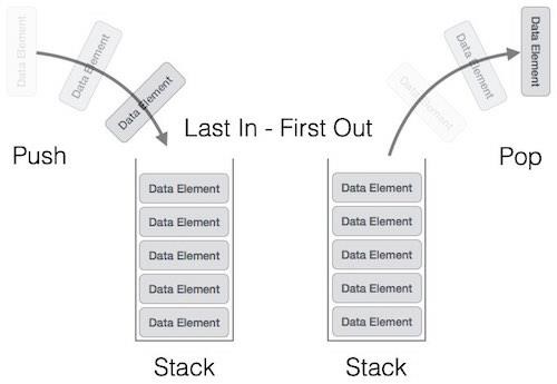
This feature makes it LIFO data structure. LIFO stands for Last-in-first-out. Here, the element which is placed (inserted or added) last, is accessed first. In stack terminology, insertion operation is called PUSH operation and removal operation is called POP operation.
Stack Representation
The following diagram depicts a stack and its operations −
A stack can be implemented by means of Array, Structure, Pointer, and Linked List. Stack can either be a fixed size one or it may have a sense of dynamic resizing. Here, we are going to implement stack using arrays, which makes it a fixed size stack implementation.
Basic Operations
Stack operations may involve initializing the stack, using it and then de-initializing it. Apart from these basic stuffs, a stack is used for the following two primary operations −
push() − Pushing (storing) an element on the stack.
pop() − Removing (accessing) an element from the stack.
When data is PUSHed onto stack.
To use a stack efficiently, we need to check the status of stack as well. For the same purpose, the following functionality is added to stacks −
peek() − get the top data element of the stack, without removing it.
isFull() − check if stack is full.
isEmpty() − check if stack is empty.
At all times, we maintain a pointer to the last PUSHed data on the stack. As this pointer always represents the top of the stack, hence named top. The top pointer provides top value of the stack without actually removing it.
First we should learn about procedures to support stack functions −
peek()
Algorithm of peek() function −
begin procedure peek
   return stack[top]
end procedure
Implementation of peek() function in C programming language −
Example
int peek() {
   return stack[top];
}
isfull()
Algorithm of isfull() function −
begin procedure isfull

   if top equals to MAXSIZE
      return true
   else
      return false
   endif

end procedure
Implementation of isfull() function in C programming language −
Example
bool isfull() {
   if(top == MAXSIZE)
      return true;
   else
      return false;
}
isempty()
Algorithm of isempty() function −
begin procedure isempty

   if top less than 1
      return true
   else
      return false
   endif

end procedure
Implementation of isempty() function in C programming language is slightly different. We initialize top at -1, as the index in array starts from 0. So we check if the top is below zero or -1 to determine if the stack is empty. Here's the code −
Example
bool isempty() {
   if(top == -1)
      return true;
   else
      return false;
}
Push Operation
The process of putting a new data element onto stack is known as a Push Operation. Push operation involves a series of steps −
Step 1 − Checks if the stack is full.
Step 2 − If the stack is full, produces an error and exit.
Step 3 − If the stack is not full, increments top to point next empty space.
Step 4 − Adds data element to the stack location, where top is pointing.
Step 5 − Returns success.
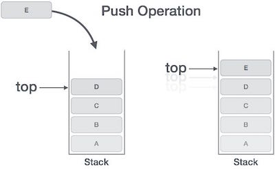
If the linked list is used to implement the stack, then in step 3, we need to allocate space dynamically.
Algorithm for PUSH Operation
A simple algorithm for Push operation can be derived as follows −
begin procedure push: stack, data

   if stack is full
      return null
   endif

   top ← top + 1
   stack[top] ← data

end procedure
Implementation of this algorithm in C, is very easy. See the following code −
Example
void push(int data) {
   if(!isFull()) {
      top = top + 1;
      stack[top] = data;
   } else {
      printf("Could not insert data, Stack is full.\n");
   }
}
Pop Operation
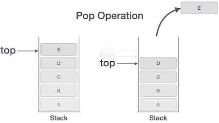
Accessing the content while removing it from the stack, is known as a Pop Operation. In an array implementation of pop() operation, the data element is not actually removed, instead top is decremented to a lower position in the stack to point to the next value. But in linked-list implementation, pop() actually removes data element and deallocates memory space.
A Pop operation may involve the following steps −
Step 1 − Checks if the stack is empty.
Step 2 − If the stack is empty, produces an error and exit.
Step 3 − If the stack is not empty, accesses the data element at which top is pointing.
Step 4 − Decreases the value of top by 1.
Step 5 − Returns success.
Algorithm for Pop Operation
A simple algorithm for Pop operation can be derived as follows −
begin procedure pop: stack

   if stack is empty
      return null
   endif

   data ← stack[top]
   top ← top - 1
   return data

end procedure
Implementation of this algorithm in C, is as follows −
Example
int pop(int data) {

   if(!isempty()) {
      data = stack[top];
      top = top - 1;
      return data;
   } else {
      printf("Could not retrieve data, Stack is empty.\n");
   }
}
The way to write arithmetic expression is known as a notation. An arithmetic expression can be written in three different but equivalent notations, i.e., without changing the essence or output of an expression. These notations are −
- Infix Notation
- Prefix (Polish) Notation
- Postfix (Reverse-Polish) Notation
These notations are named as how they use operator in expression. We shall learn the same here in this chapter.
Infix Notation
We write expression in infix notation, e.g. a - b + c, where operators are used in-between operands. It is easy for us humans to read, write, and speak in infix notation but the same does not go well with computing devices. An algorithm to process infix notation could be difficult and costly in terms of time and space consumption.
Prefix Notation
In this notation, operator is prefixed to operands, i.e. operator is written ahead of operands. For example, +ab. This is equivalent to its infix notation a + b. Prefix notation is also known as Polish Notation.
Postfix Notation
This notation style is known as Reversed Polish Notation. In this notation style, the operator is postfixed to the operands i.e., the operator is written after the operands. For example, ab+. This is equivalent to its infix notation a + b.
The following table briefly tries to show the difference in all three notations −
Sr.No. Infix Notation Prefix Notation Postfix Notation 1 a + b + a b a b + 2 (a + b) ∗ c ∗ + a b c a b + c ∗ 3 a ∗ (b + c) ∗ a + b c a b c + ∗ 4 a / b + c / d + / a b / c d a b / c d / + 5 (a + b) ∗ (c + d) ∗ + a b + c d a b + c d + ∗ 6 ((a + b) ∗ c) - d - ∗ + a b c d a b + c ∗ d -
Parsing Expressions
As we have discussed, it is not a very efficient way to design an algorithm or program to parse infix notations. Instead, these infix notations are first converted into either postfix or prefix notations and then computed.
To parse any arithmetic expression, we need to take care of operator precedence and associativity also.
Precedence
When an operand is in between two different operators, which operator will take the operand first, is decided by the precedence of an operator over others. For example −

As multiplication operation has precedence over addition, b * c will be evaluated first. A table of operator precedence is provided later.
Associativity
Associativity describes the rule where operators with the same precedence appear in an expression. For example, in expression a + b − c, both + and – have the same precedence, then which part of the expression will be evaluated first, is determined by associativity of those operators. Here, both + and − are left associative, so the expression will be evaluated as (a + b) − c.
Precedence and associativity determines the order of evaluation of an expression. Following is an operator precedence and associativity table (highest to lowest) −
Sr.No. Operator Precedence Associativity 1 Exponentiation ^ Highest Right Associative 2 Multiplication ( ∗ ) & Division ( / ) Second Highest Left Associative 3 Addition ( + ) & Subtraction ( − ) Lowest Left Associative
The above table shows the default behavior of operators. At any point of time in expression evaluation, the order can be altered by using parenthesis. For example −
In a + b*c, the expression part b*c will be evaluated first, with multiplication as precedence over addition. We here use parenthesis for a + b to be evaluated first, like (a + b)*c.
Postfix Evaluation Algorithm
We shall now look at the algorithm on how to evaluate postfix notation −
Step 1 − scan the expression from left to right
Step 2 − if it is an operand push it to stack
Step 3 − if it is an operator pull operand from stack and perform operation
Step 4 − store the output of step 3, back to stack
Step 5 − scan the expression until all operands are consumed
Step 6 − pop the stack and perform operation
Queue is an abstract data structure, somewhat similar to Stacks. Unlike stacks, a queue is open at both its ends. One end is always used to insert data (enqueue) and the other is used to remove data (dequeue). Queue follows First-In-First-Out methodology, i.e., the data item stored first will be accessed first.

A real-world example of queue can be a single-lane one-way road, where the vehicle enters first, exits first. More real-world examples can be seen as queues at the ticket windows and bus-stops.
Queue Representation
As we now understand that in queue, we access both ends for different reasons. The following diagram given below tries to explain queue representation as data structure −

As in stacks, a queue can also be implemented using Arrays, Linked-lists, Pointers and Structures. For the sake of simplicity, we shall implement queues using one-dimensional array.
Basic Operations
Queue operations may involve initializing or defining the queue, utilizing it, and then completely erasing it from the memory. Here we shall try to understand the basic operations associated with queues −
enqueue() − add (store) an item to the queue.
dequeue() − remove (access) an item from the queue.
Few more functions are required to make the above-mentioned queue operation efficient. These are −
peek() − Gets the element at the front of the queue without removing it.
isfull() − Checks if the queue is full.
isempty() − Checks if the queue is empty.
In queue, we always dequeue (or access) data, pointed by front pointer and while enqueing (or storing) data in the queue we take help of rear pointer.
Let's first learn about supportive functions of a queue −
peek()
This function helps to see the data at the front of the queue. The algorithm of peek() function is as follows −
Algorithm
begin procedure peek
return queue[front]
end procedure
Implementation of peek() function in C programming language −
Example
int peek() {
return queue[front];
}
isfull()
As we are using single dimension array to implement queue, we just check for the rear pointer to reach at MAXSIZE to determine that the queue is full. In case we maintain the queue in a circular linked-list, the algorithm will differ. Algorithm of isfull() function −
Algorithm
begin procedure isfull
if rear equals to MAXSIZE
return true
else
return false
endif
end procedure
Implementation of isfull() function in C programming language −
Example
bool isfull() {
if(rear == MAXSIZE - 1)
return true;
else
return false;
}
isempty()
Algorithm of isempty() function −
Algorithm
begin procedure isempty
if front is less than MIN OR front is greater than rear
return true
else
return false
endif
end procedure
If the value of front is less than MIN or 0, it tells that the queue is not yet initialized, hence empty.
Here's the C programming code −
Example
bool isempty() {
if(front < 0 || front > rear)
return true;
else
return false;
}
Enqueue Operation
Queues maintain two data pointers, front and rear. Therefore, its operations are comparatively difficult to implement than that of stacks.
The following steps should be taken to enqueue (insert) data into a queue −
Step 1 − Check if the queue is full.
Step 2 − If the queue is full, produce overflow error and exit.
Step 3 − If the queue is not full, increment rear pointer to point the next empty space.
Step 4 − Add data element to the queue location, where the rear is pointing.
Step 5 − return success.
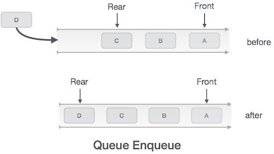
Sometimes, we also check to see if a queue is initialized or not, to handle any unforeseen situations.
Algorithm for enqueue operation
procedure enqueue(data)
if queue is full
return overflow
endif
rear ← rear + 1
queue[rear] ← data
return true
end procedure
Implementation of enqueue() in C programming language −
Example
int enqueue(int data)
if(isfull())
return 0;
rear = rear + 1;
queue[rear] = data;
return 1;
end procedure
Dequeue Operation
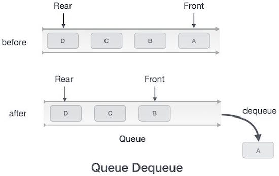
Accessing data from the queue is a process of two tasks − access the data where front is pointing and remove the data after access. The following steps are taken to perform dequeue operation −
Step 1 − Check if the queue is empty.
Step 2 − If the queue is empty, produce underflow error and exit.
Step 3 − If the queue is not empty, access the data where front is pointing.
Step 4 − Increment front pointer to point to the next available data element.
Step 5 − Return success.
Algorithm for dequeue operation
procedure dequeue
if queue is empty
return underflow
end if
data = queue[front]
front ← front + 1
return true
end procedure
Implementation of dequeue() in C programming language −
Example
int dequeue() {
if(isempty())
return 0;
int data = queue[front];
front = front + 1;
return data;
}
Linear search is a very simple search algorithm. In this type of search, a sequential search is made over all items one by one. Every item is checked and if a match is found then that particular item is returned, otherwise the search continues till the end of the data collection.
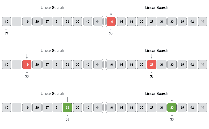
Algorithm
Linear Search ( Array A, Value x)
Step 1: Set i to 1
Step 2: if i > n then go to step 7
Step 3: if A[i] = x then go to step 6
Step 4: Set i to i + 1
Step 5: Go to Step 2
Step 6: Print Element x Found at index i and go to step 8
Step 7: Print element not found
Step 8: Exit
Pseudocode
procedure linear_search (list, value)
for each item in the list
if match item == value
return the item's location
end if
end for
end procedure
Binary search is a fast search algorithm with run-time complexity of Ο(log n). This search algorithm works on the principle of divide and conquer. For this algorithm to work properly, the data collection should be in the sorted form.
Binary search looks for a particular item by comparing the middle most item of the collection. If a match occurs, then the index of item is returned. If the middle item is greater than the item, then the item is searched in the sub-array to the left of the middle item. Otherwise, the item is searched for in the sub-array to the right of the middle item. This process continues on the sub-array as well until the size of the subarray reduces to zero.
How Binary Search Works?
For a binary search to work, it is mandatory for the target array to be sorted. We shall learn the process of binary search with a pictorial example. The following is our sorted array and let us assume that we need to search the location of value 31 using binary search.

First, we shall determine half of the array by using this formula −
mid = low + (high - low) / 2
Here it is, 0 + (9 - 0 ) / 2 = 4 (integer value of 4.5). So, 4 is the mid of the array.

Now we compare the value stored at location 4, with the value being searched, i.e. 31. We find that the value at location 4 is 27, which is not a match. As the value is greater than 27 and we have a sorted array, so we also know that the target value must be in the upper portion of the array.

We change our low to mid + 1 and find the new mid value again.
low = mid + 1
mid = low + (high - low) / 2
Our new mid is 7 now. We compare the value stored at location 7 with our target value 31.

The value stored at location 7 is not a match, rather it is more than what we are looking for. So, the value must be in the lower part from this location.

Hence, we calculate the mid again. This time it is 5.

We compare the value stored at location 5 with our target value. We find that it is a match.

We conclude that the target value 31 is stored at location 5.
Binary search halves the searchable items and thus reduces the count of comparisons to be made to very less numbers.
Pseudocode
The pseudocode of binary search algorithms should look like this −
Procedure binary_search
A ← sorted array
n ← size of array
x ← value to be searched
Set lowerBound = 1
Set upperBound = n
while x not found
if upperBound < lowerBound
EXIT: x does not exists.
set midPoint = lowerBound + ( upperBound - lowerBound ) / 2
if A[midPoint] < x
set lowerBound = midPoint + 1
if A[midPoint] > x
set upperBound = midPoint - 1
if A[midPoint] = x
EXIT: x found at location midPoint
end while
end procedure
Interpolation search is an improved variant of binary search. This search algorithm works on the probing position of the required value. For this algorithm to work properly, the data collection should be in a sorted form and equally distributed.
Binary search has a huge advantage of time complexity over linear search. Linear search has worst-case complexity of Ο(n) whereas binary search has Ο(log n).
There are cases where the location of target data may be known in advance. For example, in case of a telephone directory, if we want to search the telephone number of Morphius. Here, linear search and even binary search will seem slow as we can directly jump to memory space where the names start from 'M' are stored.
Positioning in Binary Search
In binary search, if the desired data is not found then the rest of the list is divided in two parts, lower and higher. The search is carried out in either of them.


Even when the data is sorted, binary search does not take advantage to probe the position of the desired data.
Position Probing in Interpolation Search
Interpolation search finds a particular item by computing the probe position. Initially, the probe position is the position of the middle most item of the collection.


If a match occurs, then the index of the item is returned. To split the list into two parts, we use the following method −
mid = Lo + ((Hi - Lo) / (A[Hi] - A[Lo])) * (X - A[Lo])
where −
A = list
Lo = Lowest index of the list
Hi = Highest index of the list
A[n] = Value stored at index n in the list
If the middle item is greater than the item, then the probe position is again calculated in the sub-array to the right of the middle item. Otherwise, the item is searched in the subarray to the left of the middle item. This process continues on the sub-array as well until the size of subarray reduces to zero.
Runtime complexity of interpolation search algorithm is Ο(log (log n)) as compared to Ο(log n) of BST in favorable situations.
Algorithm
As it is an improvisation of the existing BST algorithm, we are mentioning the steps to search the 'target' data value index, using position probing −
Step 1 − Start searching data from middle of the list.
Step 2 − If it is a match, return the index of the item, and exit.
Step 3 − If it is not a match, probe position.
Step 4 − Divide the list using probing formula and find the new midle.
Step 5 − If data is greater than middle, search in higher sub-list.
Step 6 − If data is smaller than middle, search in lower sub-list.
Step 7 − Repeat until match.
Pseudocode
A → Array list
N → Size of A
X → Target Value
Procedure Interpolation_Search()
Set Lo → 0
Set Mid → -1
Set Hi → N-1
While X does not match
if Lo equals to Hi OR A[Lo] equals to A[Hi]
EXIT: Failure, Target not found
end if
Set Mid = Lo + ((Hi - Lo) / (A[Hi] - A[Lo])) * (X - A[Lo])
if A[Mid] = X
EXIT: Success, Target found at Mid
else
if A[Mid] < X
Set Lo to Mid+1
else if A[Mid] > X
Set Hi to Mid-1
end if
end if
End While
End Procedure
Hash Table is a data structure which stores data in an associative manner. In a hash table, data is stored in an array format, where each data value has its own unique index value. Access of data becomes very fast if we know the index of the desired data.
Thus, it becomes a data structure in which insertion and search operations are very fast irrespective of the size of the data. Hash Table uses an array as a storage medium and uses hash technique to generate an index where an element is to be inserted or is to be located from.
Hashing
Hashing is a technique to convert a range of key values into a range of indexes of an array. We're going to use modulo operator to get a range of key values. Consider an example of hash table of size 20, and the following items are to be stored. Item are in the (key,value) format.

- (1,20)
- (2,70)
- (42,80)
- (4,25)
- (12,44)
- (14,32)
- (17,11)
- (13,78)
- (37,98)
Sr.No. Key Hash Array Index 1 1 1 % 20 = 1 1 2 2 2 % 20 = 2 2 3 42 42 % 20 = 2 2 4 4 4 % 20 = 4 4 5 12 12 % 20 = 12 12 6 14 14 % 20 = 14 14 7 17 17 % 20 = 17 17 8 13 13 % 20 = 13 13 9 37 37 % 20 = 17 17
Linear Probing
As we can see, it may happen that the hashing technique is used to create an already used index of the array. In such a case, we can search the next empty location in the array by looking into the next cell until we find an empty cell. This technique is called linear probing.
Sr.No. Key Hash Array Index After Linear Probing, Array Index 1 1 1 % 20 = 1 1 1 2 2 2 % 20 = 2 2 2 3 42 42 % 20 = 2 2 3 4 4 4 % 20 = 4 4 4 5 12 12 % 20 = 12 12 12 6 14 14 % 20 = 14 14 14 7 17 17 % 20 = 17 17 17 8 13 13 % 20 = 13 13 13 9 37 37 % 20 = 17 17 18
Basic Operations
Following are the basic primary operations of a hash table.
Search − Searches an element in a hash table.
Insert − inserts an element in a hash table.
delete − Deletes an element from a hash table.
DataItem
Define a data item having some data and key, based on which the search is to be conducted in a hash table.
struct DataItem {
int data;
int key;
};
Hash Method
Define a hashing method to compute the hash code of the key of the data item.
int hashCode(int key){
return key % SIZE;
}
Search Operation
Whenever an element is to be searched, compute the hash code of the key passed and locate the element using that hash code as index in the array. Use linear probing to get the element ahead if the element is not found at the computed hash code.
Example
struct DataItem *search(int key) {
//get the hash
int hashIndex = hashCode(key);
//move in array until an empty
while(hashArray[hashIndex] != NULL) {
if(hashArray[hashIndex]->key == key)
return hashArray[hashIndex];
//go to next cell
++hashIndex;
//wrap around the table
hashIndex %= SIZE;
}
return NULL;
}
Insert Operation
Whenever an element is to be inserted, compute the hash code of the key passed and locate the index using that hash code as an index in the array. Use linear probing for empty location, if an element is found at the computed hash code.
Example
void insert(int key,int data) {
struct DataItem *item = (struct DataItem*) malloc(sizeof(struct DataItem));
item->data = data;
item->key = key;
//get the hash
int hashIndex = hashCode(key);
//move in array until an empty or deleted cell
while(hashArray[hashIndex] != NULL && hashArray[hashIndex]->key != -1) {
//go to next cell
++hashIndex;
//wrap around the table
hashIndex %= SIZE;
}
hashArray[hashIndex] = item;
}
Delete Operation
Whenever an element is to be deleted, compute the hash code of the key passed and locate the index using that hash code as an index in the array. Use linear probing to get the element ahead if an element is not found at the computed hash code. When found, store a dummy item there to keep the performance of the hash table intact.
Example
struct DataItem* delete(struct DataItem* item) {
int key = item->key;
//get the hash
int hashIndex = hashCode(key);
//move in array until an empty
while(hashArray[hashIndex] !=NULL) {
if(hashArray[hashIndex]->key == key) {
struct DataItem* temp = hashArray[hashIndex];
//assign a dummy item at deleted position
hashArray[hashIndex] = dummyItem;
return temp;
}
//go to next cell
++hashIndex;
//wrap around the table
hashIndex %= SIZE;
}
return NULL;
}
Sorting refers to arranging data in a particular format. Sorting algorithm specifies the way to arrange data in a particular order. Most common orders are in numerical or lexicographical order.
The importance of sorting lies in the fact that data searching can be optimized to a very high level, if data is stored in a sorted manner. Sorting is also used to represent data in more readable formats. Following are some of the examples of sorting in real-life scenarios −
Telephone Directory − The telephone directory stores the telephone numbers of people sorted by their names, so that the names can be searched easily.
Dictionary − The dictionary stores words in an alphabetical order so that searching of any word becomes easy.
In-place Sorting and Not-in-place Sorting
Sorting algorithms may require some extra space for comparison and temporary storage of few data elements. These algorithms do not require any extra space and sorting is said to happen in-place, or for example, within the array itself. This is called in-place sorting. Bubble sort is an example of in-place sorting.
However, in some sorting algorithms, the program requires space which is more than or equal to the elements being sorted. Sorting which uses equal or more space is called not-in-place sorting. Merge-sort is an example of not-in-place sorting.
Stable and Not Stable Sorting
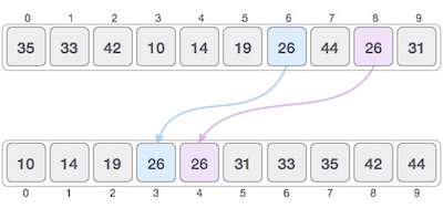
If a sorting algorithm, after sorting the contents, does not change the sequence of similar content in which they appear, it is called stable sorting.
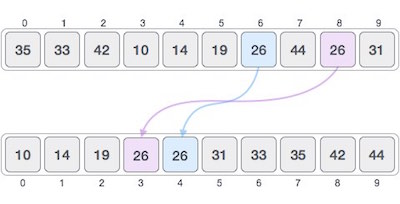
If a sorting algorithm, after sorting the contents, changes the sequence of similar content in which they appear, it is called unstable sorting.
Stability of an algorithm matters when we wish to maintain the sequence of original elements, like in a tuple for example.
Adaptive and Non-Adaptive Sorting Algorithm
A sorting algorithm is said to be adaptive, if it takes advantage of already 'sorted' elements in the list that is to be sorted. That is, while sorting if the source list has some element already sorted, adaptive algorithms will take this into account and will try not to re-order them.
A non-adaptive algorithm is one which does not take into account the elements which are already sorted. They try to force every single element to be re-ordered to confirm their sortedness.
Important Terms
Some terms are generally coined while discussing sorting techniques, here is a brief introduction to them −
Increasing Order
A sequence of values is said to be in increasing order, if the successive element is greater than the previous one. For example, 1, 3, 4, 6, 8, 9 are in increasing order, as every next element is greater than the previous element.
Decreasing Order
A sequence of values is said to be in decreasing order, if the successive element is less than the current one. For example, 9, 8, 6, 4, 3, 1 are in decreasing order, as every next element is less than the previous element.
Non-Increasing Order
A sequence of values is said to be in non-increasing order, if the successive element is less than or equal to its previous element in the sequence. This order occurs when the sequence contains duplicate values. For example, 9, 8, 6, 3, 3, 1 are in non-increasing order, as every next element is less than or equal to (in case of 3) but not greater than any previous element.
Non-Decreasing Order
A sequence of values is said to be in non-decreasing order, if the successive element is greater than or equal to its previous element in the sequence. This order occurs when the sequence contains duplicate values. For example, 1, 3, 3, 6, 8, 9 are in non-decreasing order, as every next element is greater than or equal to (in case of 3) but not less than the previous one.

Comments
Post a Comment